Quality control of sc/snRNA-seq
Mariano Ruz Jurado
Goethe UniversitySource:
vignettes/DOtools.Rmd
DOtools.RmdInstallation
DOtools is an R package distributed as part of the Bioconductor project. To install the package, start R and enter:
install.packages("BiocManager")
BiocManager::install("DOtools")
Alternatively, you can instead install the latest development version from GitHub with:
BiocManager::install("MarianoRuzJurado/DOtools")Usage
DOtools contains different functions for processing and visualizing gene expression in scRNA/snRNA experiments:
In this vignette we showcase how to use the functions with public
available data. We recommend using the build-in logging in R with
sink().
Libraries
DOtools can be imported as:
Ambient removal
Despite advances in optimizing and standardizing droplet-based single-cell omics protocols like single-cell and single-nucleus RNA sequencing (sc/snRNA-seq), these experiments still suffer from systematic biases and background noise. In particular, ambient RNA in snRNA-seq can lead to an overestimation of expression levels for certain genes. Computational tools such as cellbender have been developed to address these biases by correcting for ambient RNA contamination.
We have integrated a wrapper function to run CellBender within the DOtools package. The current implementation supports processing samples generated with CellRanger.
base <- DOtools:::.example_10x()
dir.create(file.path(base, "/cellbender"))

raw_files <- list.files(base,
    pattern = "raw_feature_bc_matrix\\.h5$",
    recursive = TRUE,
    full.names = TRUE
)

DO.CellBender(
    cellranger_path = base,
    output_path = file.path(base, "/cellbender"),
    samplenames = c("disease"),
    cuda = TRUE,
    BarcodeRanking = FALSE,
    cpu_threads = 48,
    epochs = 150
)
After running the analysis, several files are saved in the
output_folder, including a summary report to check for any
issues during CellBender execution, individual log files for each
sample, and a commands_Cellbender.txt file with the exact
command used. The corrected .h5 files can then be used
alternatively to the cellranger output for downstream analysis.
Quality control
DOtools
The DO.Import() function provides a streamlined pipeline
for performing quality control on single-cell or single-nucleus RNA
sequencing (sc/snRNA-seq) data. It takes as input a list of .h5 files
generated by e.g. CellRanger or STARsolo, along with sample names and
metadata.
During preprocessing, low-quality genes and cells are filtered out based on specified thresholds. Genes expressed in fewer than five cells are removed. Cells are filtered according to mitochondrial gene content, number of detected genes, total UMI counts, and potential doublets. The function supports doublet detection using scDblFinder. Thresholds for mitochondrial content (e.g., 5% for scRNA-seq and 3% for snRNA-seq), gene counts, and UMI counts can be defined to tailor the filtering.
After filtering, samples are merged into one SingleCellExperiment or Seurat object, followed by log-normalisation, scaling, and the identification of highly variable genes. To help assess the effect of quality control, violin plots showing distributions of key metrics before and after filtering are automatically generated and saved alongside the input files. A summary of removed genes and cells is also recorded.
To show how the quality control works, we are going to use a public dataset from 10X from human blood of healthy and donors with a malignant tumor:
base <- DOtools:::.example_10x()

paths <- c(
    file.path(base, "healthy/outs/filtered_feature_bc_matrix.h5"),
    file.path(base, "disease/outs/filtered_feature_bc_matrix.h5")
)

SCE_obj <- DO.Import(
    pathways = paths,
    ids = c("healthy-1", "disease-1"),
    DeleteDoublets = TRUE,
    cut_mt = .05,
    min_counts = 500,
    min_genes = 300,
    high_quantile = .95,
    Seurat = FALSE # Set to TRUE for Seurat object
)
We can now check the quality before introducing filterings:
prefilterplots <- system.file(
    "figures", "prefilterplots-1.png",
    package = "DOtools"
)

pQC1 <- magick::image_read(prefilterplots)
plot(pQC1)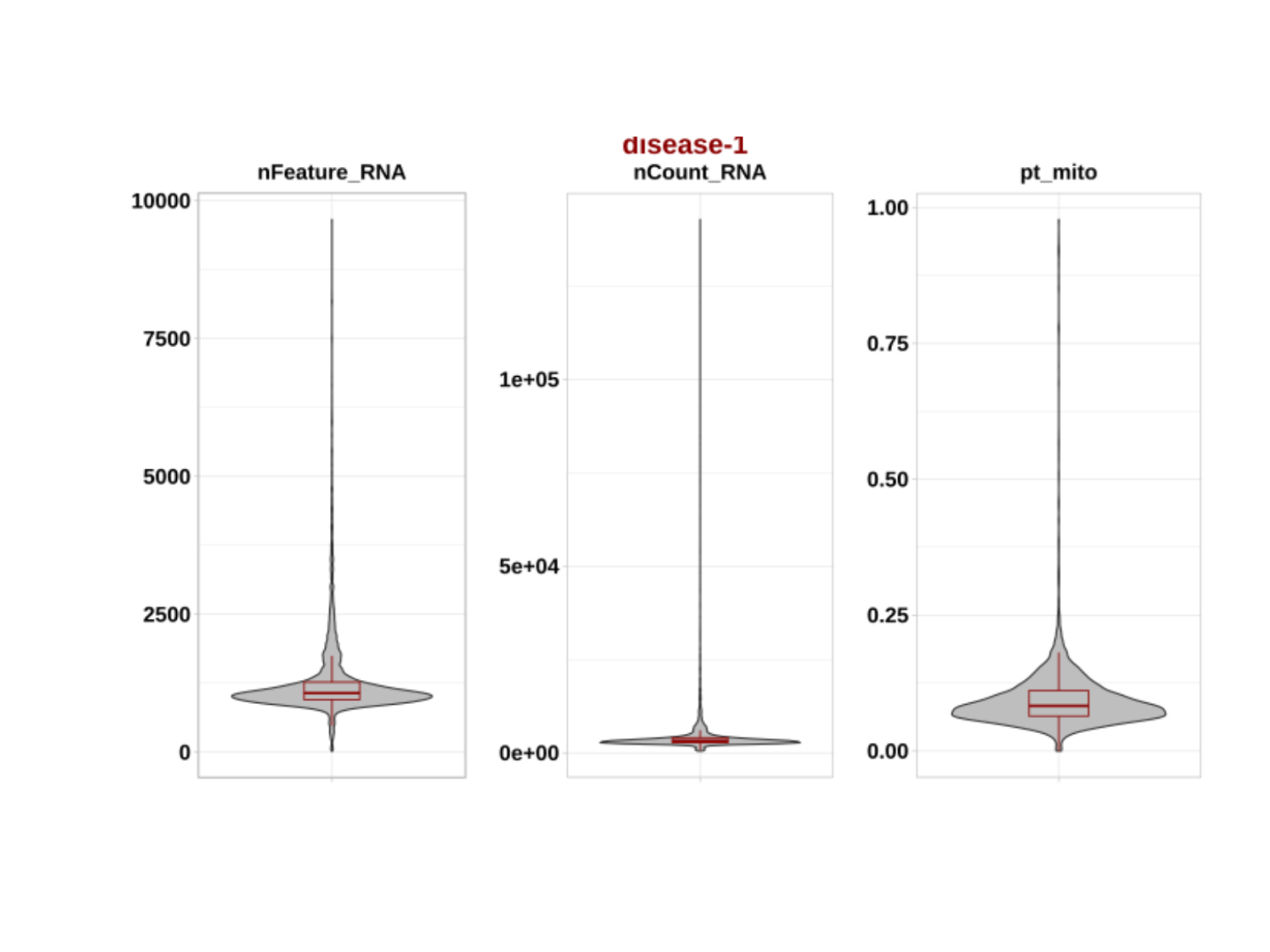
And after:
postfilterplots <- system.file(
"figures",
"postfilterplots-1.png",
package = "DOtools"
)
pQC2 <- magick::image_read(postfilterplots)
plot(pQC2)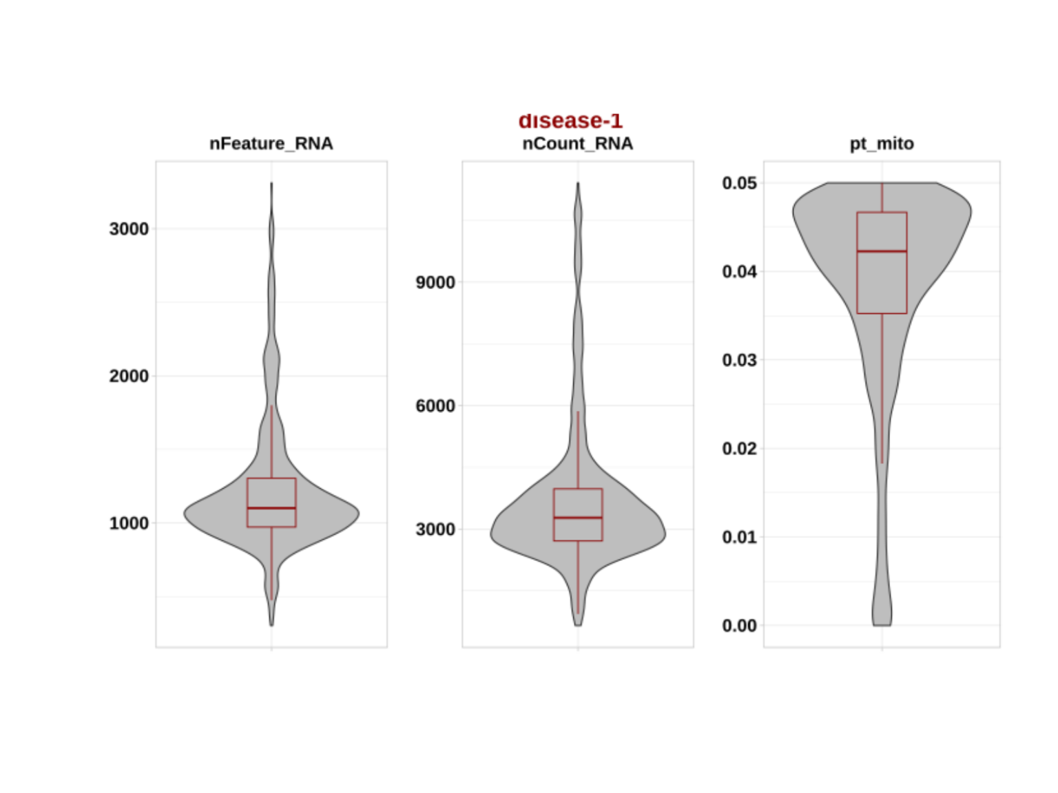 We observed that most cells were removed due to increased mitochondrial
content. Depending on the experimental design, the mitochondrial content
threshold can be adjusted to retain a higher number of cells, if
minimizing cell loss is of relevance.
We observed that most cells were removed due to increased mitochondrial
content. Depending on the experimental design, the mitochondrial content
threshold can be adjusted to retain a higher number of cells, if
minimizing cell loss is of relevance.
The DOtools package provides a slim object of this data set.
Please feel free, to use the one created from DO.Import for prettier
results or this slim downed version. We can observe how similar the
samples are through running a correlation analysis.
# Making sure we have a save folder
base <- tempfile("my_tempdir_")
dir.create(base)

SCE_obj <- readRDS(
    system.file("extdata",
        "sce_data.rds",
        package = "DOtools"
    )
)

DO.Correlation(SCE_obj)
#> Warning: `aes_string()` was deprecated in ggplot2 3.0.0.
#> ℹ Please use tidy evaluation idioms with `aes()`.
#> ℹ See also `vignette("ggplot2-in-packages")` for more information.
#> ℹ The deprecated feature was likely used in the ggcorrplot package.
#>   Please report the issue at <https://github.com/kassambara/ggcorrplot/issues>.
#> This warning is displayed once per session.
#> Call `lifecycle::last_lifecycle_warnings()` to see where this warning was
#> generated.
#> Scale for fill is already present.
#> Adding another scale for fill, which will replace the existing scale.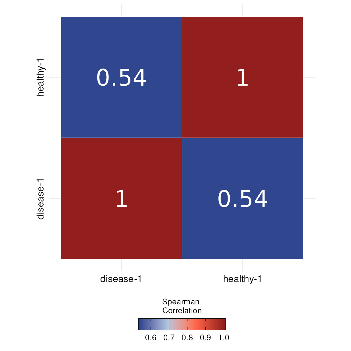
Data integration
After quality control the preferred integration method can be chosen,
we support every integration method within Seurat’s
IntegrateLayers function. Additionally, we implemented a
new wrapper function for the scVI integration from the scvi-tools package.
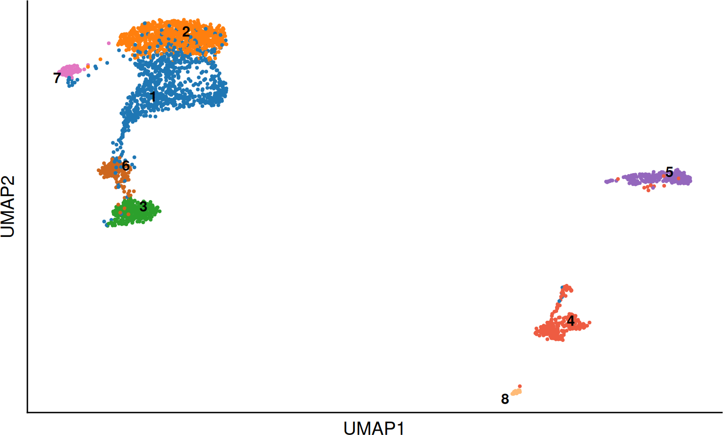
After the integration completes, we run the Leiden algorithm to find
clusters and generate UMAP embeddings.
SCE_obj <- DO.Integration(
    sce_object = SCE_obj,
    split_key = "orig.ident",
    HVG = TRUE,
    scale = TRUE,
    pca = TRUE,
    integration_method = "CCAIntegration"
)
#> 2026-06-12 10:54:37 - Splitting object for integration with CCAIntegration by orig.ident
#> 2026-06-12 10:54:37 - Calculating highly variable genes
#> 2026-06-12 10:54:37 - Scaling object
#> 2026-06-12 10:54:37 - Running pca, saved in key: PCA
#> Splitting 'counts', 'data' layers. Not splitting 'scale.data'. If you would like to split other layers, set in `layers` argument.
#> 2026-06-12 10:54:38 - Running integration, saved in key: INTEGRATED.CCA
#> 2026-06-12 10:54:43 - Running Nearest-neighbor graph construction
#> 2026-06-12 10:54:44 - Running cluster detection
#> 2026-06-12 10:54:44 - Creating UMAP
# (Optional) Integration with scVI-Model
SCE_obj <- DO.scVI(
    sce_object = SCE_obj,
    batch_key = "orig.ident",
    layer_counts = "counts",
    layer_logcounts = "logcounts"
)


SNN_Graph <- scran::buildSNNGraph(SCE_obj,
    use.dimred = "scVI"
)

clust_SCVI <- igraph::cluster_louvain(SNN_Graph,
    resolution = 0.3
)

SCE_obj$leiden0.3 <- factor(igraph::membership(clust_SCVI))
SCE_obj <- scater::runUMAP(SCE_obj, dimred = "scVI", name = "UMAP")
After the integration finished, both corrected expression matrices can be found saved in the SCE object and can be used for cluster calculations and UMAP projections. In this case, we will continue with the CCA Integration method.
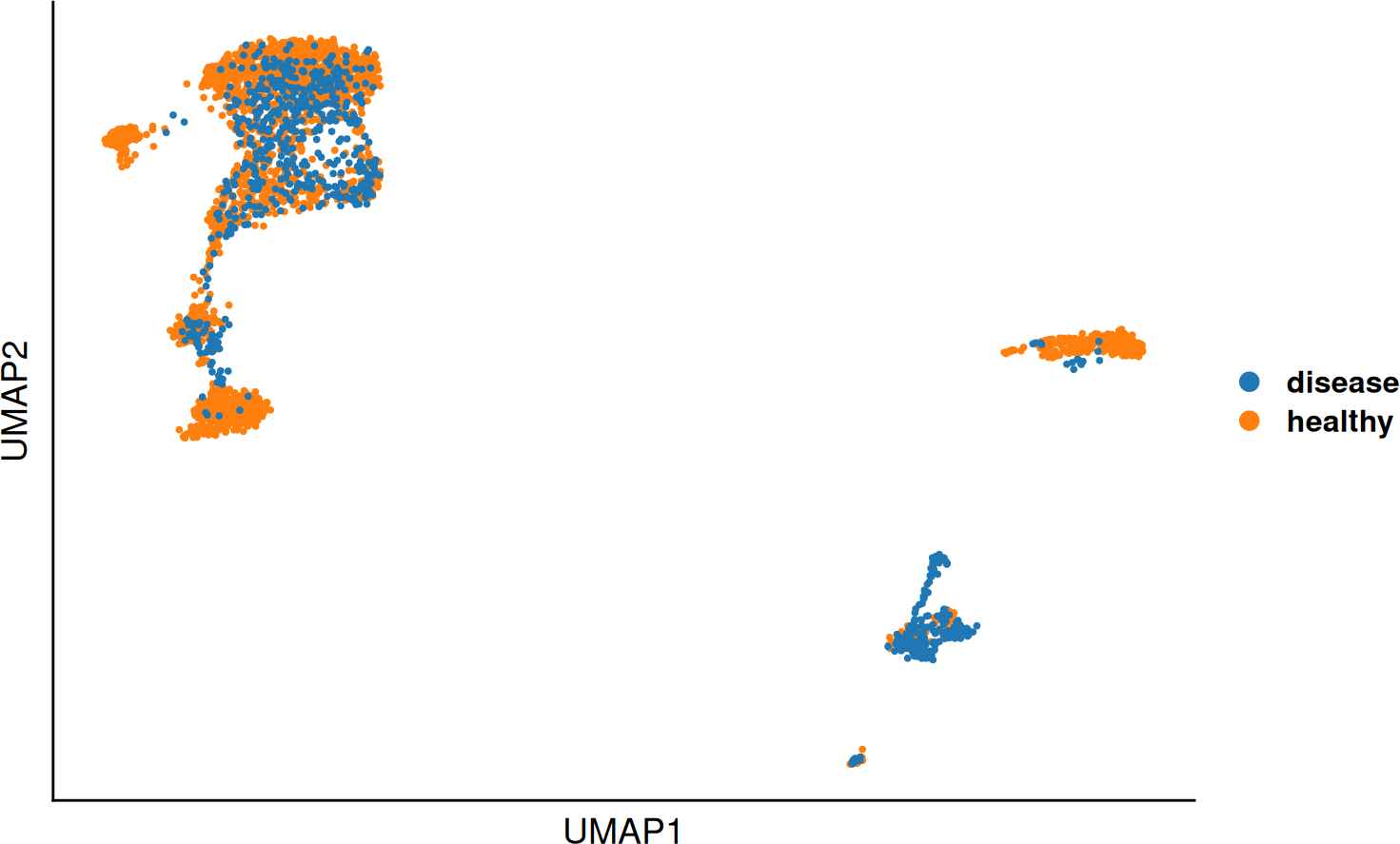
DO.UMAP(SCE_obj,
    group.by = "leiden0.3"
)
DO.UMAP(SCE_obj,
    group.by = "condition",
    legend.position = "right",
    label = FALSE
)
Semi-automatic annotation with Celltypist
Next up, we implemented a wrapper around the semi-automatic
annotation tool celltypist. It
will annotate the defined clusters based on the
Adult_COVID19_PBMC.pkl model.
SCE_obj <- DO.CellTypist(SCE_obj,
    modelName = "Healthy_COVID19_PBMC.pkl",
    runCelltypistUpdate = TRUE,
    over_clustering = "leiden0.3"
)
#> 2026-06-12 10:54:53 - Running celltypist using model: Healthy_COVID19_PBMC.pkl
#> 2026-06-12 10:54:53 - Saving celltypist results to temporary folder: /tmp/RtmpwHWUug/fileea18925e1f4
#> For native R and reading and writing of H5AD files, an R <AnnData> object, and
#> conversion to <SingleCellExperiment> or <Seurat> objects, check out the
#> anndataR package:
#> ℹ Install it from Bioconductor with `BiocManager::install("anndataR")`
#> ℹ See more at <https://bioconductor.org/packages/anndataR/>
#> 2026-06-12 10:55:11 - Creating probality plot
#>
#> This message is displayed once per session.
DO.UMAP(SCE_obj, group.by = "autoAnnot", legend.position = "right")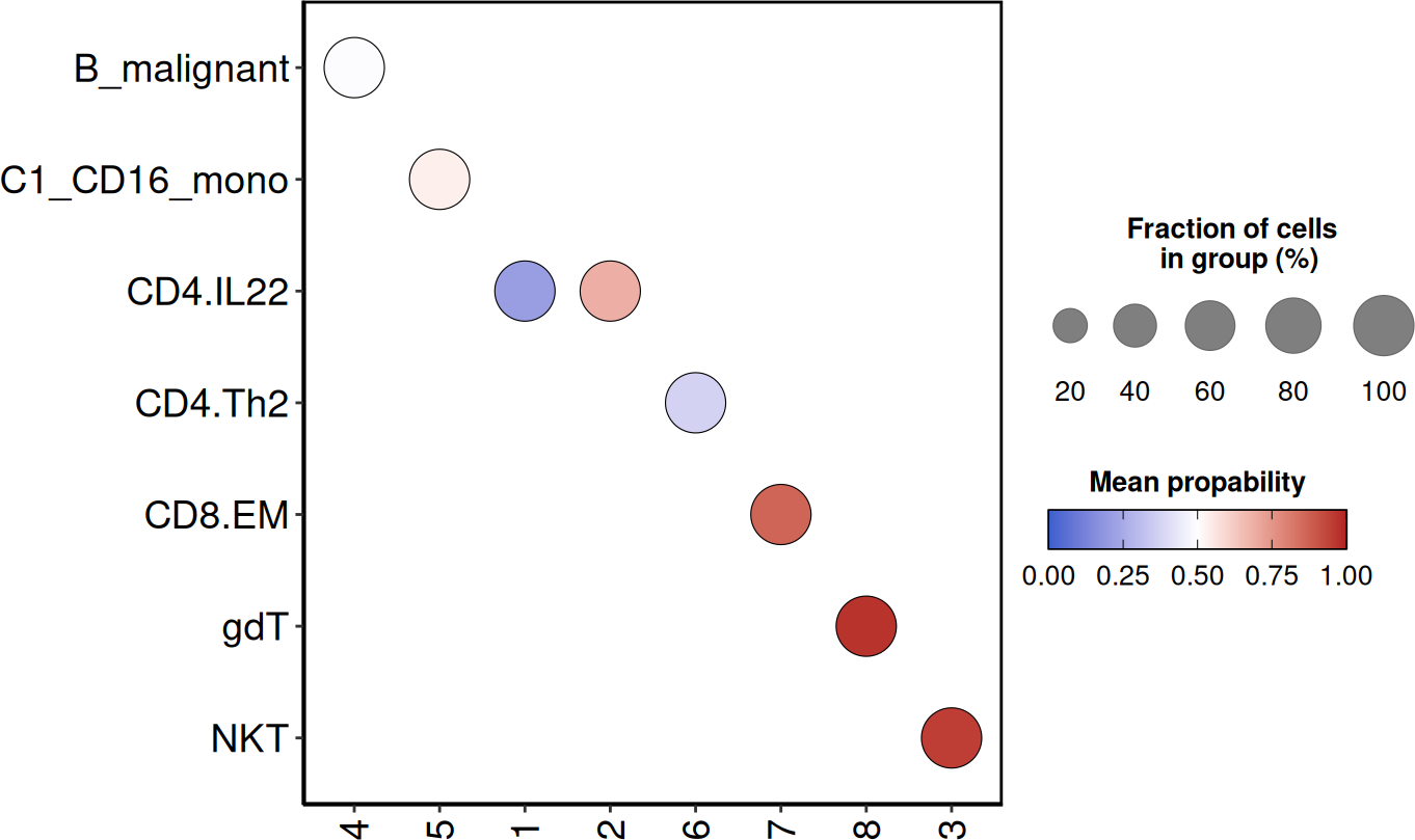
The semi-automatic annotation is a good estimate of the cell types in
your object. But you should always manually validate the findings of the
model. You can manually define a set of marker genes for the cell
population or check the most preeminent genes per cluster by using
scran’s findMarkers function. Marker genes can also be
visualised using the DO.UMAP function.
markers_list <- scran::findMarkers(
    SCE_obj,
    test.type = "t",
    groups = SingleCellExperiment::colData(SCE_obj)$autoAnnot,
    direction = "up",
    lfc = 0.25,
    pval.type = "any"
)
#> Warning in .findMarkers(assay(x, i = assay.type), ...): 'findMarkers' is deprecated.
#> Use 'scrapper::scoreMarkers.se' instead.
#> See help("Deprecated")
#> Warning in .local(x, ...): 'pairwiseTTests' is deprecated.
#> See help("Deprecated")
#> Warning in combineMarkers(fit$statistics, fit$pairs, pval.type = pval.type, : 'combineMarkers' is deprecated.
#> Use 'scrapper::summarizeEffects' instead.
#> See help("Deprecated")

# pick top 5 per cluster, naming adjustments
annotation_Markers <- lapply(names(markers_list), function(cluster) {
    df <- as.data.frame(markers_list[[cluster]])
    df$gene <- rownames(df)
    df$cluster <- cluster
    df %>%
        rename(
            avg_log2FC = summary.logFC,
            p_val      = p.value,
            p_val_adj  = FDR
        ) %>%
        dplyr::select(gene, cluster, avg_log2FC, p_val, p_val_adj)
}) %>%
    bind_rows()

# or with seurat if preferred
Seu_obj <- as.Seurat(SCE_obj)
annotation_Markers <- FindAllMarkers(
    object = Seu_obj,
    assay = "RNA",
    group.by = "autoAnnot",
    min.pct = 0.25,
    logfc.threshold = 0.25
)
#> Calculating cluster CD83_CD14_mono
#> For a (much!) faster implementation of the Wilcoxon Rank Sum Test,
#> (default method for FindMarkers) please install the presto package
#> --------------------------------------------
#> install.packages('devtools')
#> devtools::install_github('immunogenomics/presto')
#> --------------------------------------------
#> After installation of presto, Seurat will automatically use the more
#> efficient implementation (no further action necessary).
#> This message will be shown once per session
#> Calculating cluster CD4.Naive
#> Calculating cluster CD8.Naive
#> Calculating cluster NK_16hi
#> Calculating cluster CD8.EM
#> Calculating cluster B_naive
#> Calculating cluster pDC

annotation_Markers <- annotation_Markers %>%
    arrange(desc(avg_log2FC)) %>%
    distinct(gene, .keep_all = TRUE) %>%
    group_by(cluster) %>%
    slice_head(n = 5)

p1 <- DO.Dotplot(
    sce_object = SCE_obj,
    Feature = annotation_Markers,
    group.by.x = "leiden0.3",
    plot.margin = c(1, 1, 1, 1),
    annotation_x = TRUE,
    point_stroke = 0.1,
    annotation_x_rev = TRUE,
    textSize = 14,
    hjust = 0.5,
    vjust = 0,
    textRot = 0,
    segWidth = 0.3,
    lwd = 3
)
#> Scale for size is already present.
#> Adding another scale for size, which will replace the existing scale.
p1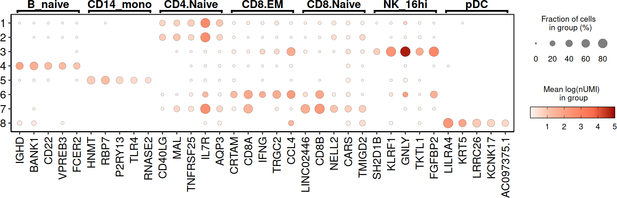
# manual set of markers
annotation_Markers <- data.frame(
    cluster = c(
        "ImmuneCells",
        rep("B_cells", 3),
        rep("T_cells", 3),
        rep("NK", 2),
        rep("Myeloid", 3),
        rep("pDC", 3)
    ),
    genes = c(
        "PTPRC", "CD79A", "BANK1", "MS4A1",
        "CD3E", "CD4", "IL7R", "NKG7",
        "KLRD1", "CD68", "CD14", "ITGAM",
        "LILRA4", "CLEC4C", "LRRC26"
    )
)

p2 <- DO.Dotplot(
    sce_object = SCE_obj,
    Feature = annotation_Markers,
    group.by.x = "leiden0.3",
    plot.margin = c(1, 1, 1, 1),
    annotation_x = TRUE,
    point_stroke = 0.1,
    annotation_x_rev = TRUE,
    textSize = 14,
    hjust = 0.5,
    vjust = 0,
    textRot = 0,
    segWidth = 0.3,
    lwd = 3
)
#> Scale for size is already present.
#> Adding another scale for size, which will replace the existing scale.
p2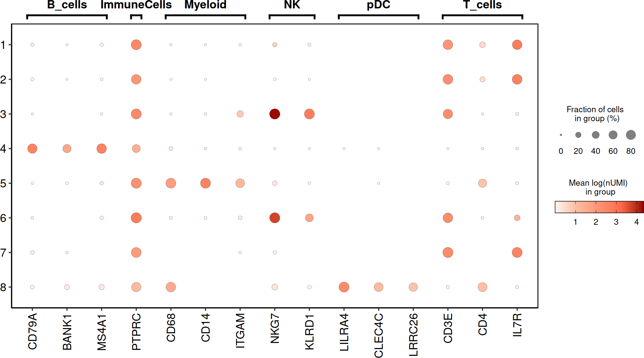
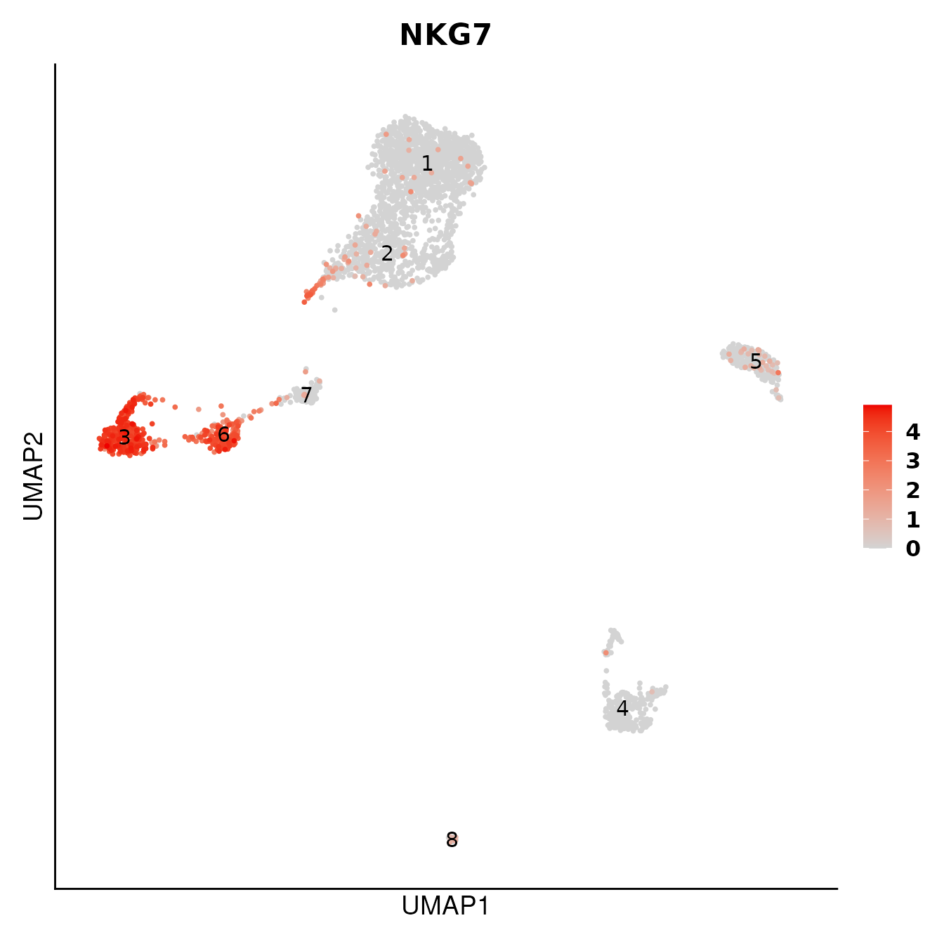
# Visualise marker expression in UMAP
DO.UMAP(SCE_obj,
    FeaturePlot = TRUE,
    features = "NKG7",
    group.by = "leiden0.3",
    legend.position = "right"
)
DO.UMAP(SCE_obj,
    DensityPlot = TRUE,
    features = "NKG7",
    group.by = "leiden0.3",
    legend.position = "right"
)
#> Warning: Removed 11400 rows containing non-finite outside the scale range
#> (`stat_contour_filled()`).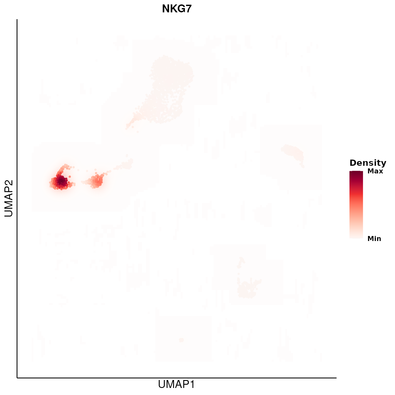
The manual markers for the immune cells show an agreement for the annotation therefore we can continue with it after some minor adjustments.
SCE_obj$annotation <- plyr::revalue(SCE_obj$leiden0.3, c(
    `1` = "T_cells",
    `2` = "T_cells",
    `3` = "NK",
    `4` = "B_cells",
    `5` = "Monocytes",
    `6` = "NK",
    `7` = "T_cells",
    `8` = "pDC"
))

DO.UMAP(SCE_obj, group.by = "annotation", legend.position = "right")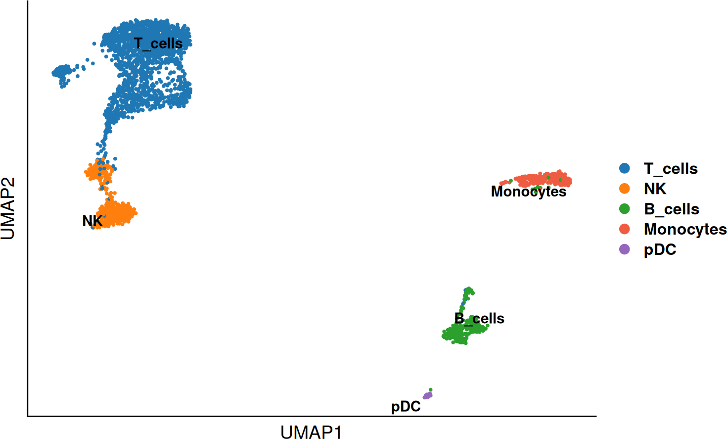
Cell composition
After the identification of the celltype populations, we can also evaluate if there are significant changes in these populations in the healthy and diseased condition using a wrapper function around the python tool scanpro.
DO.CellComposition(SCE_obj,
    assay_normalized = "RNA",
    cluster_column = "annotation",
    sample_column = "orig.ident",
    condition_column = "condition",
    transform_method = "arcsin",
    n_reps = 3
)
#> 2026-06-12 10:55:26 - Bootstrapping method activated with 3 simulated replicates!
#> .
#> Using orig.ident, condition as id variables
#> Using condition as id variables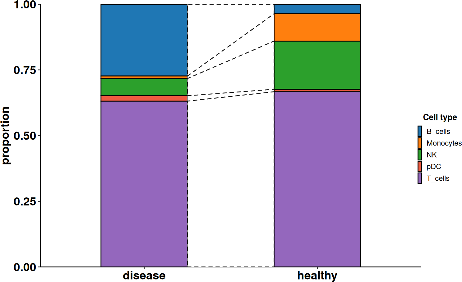
Reclustering of cell populations
Subpopulations can be tricky to find, therefore it is always a good practice to perform a reclustering of a given cell populations, if we are interested in a specific set of cells in a population. Here for example in the T cells. We will identify the subpopulations and then markers defining them.
SCE_obj <- DO.FullRecluster(SCE_obj, over_clustering = "annotation")
#> Computing nearest neighbor graph
#> Computing SNN
#> 1 singletons identified. 2 final clusters.
#> 1 singletons identified. 3 final clusters.
#>
DO.UMAP(SCE_obj, group.by = "annotation_recluster")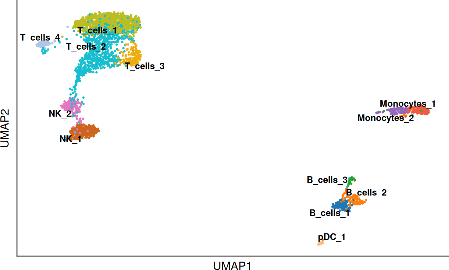
T_cells <- DO.Subset(SCE_obj,
    ident = "annotation_recluster",
    ident_name = grep("T_cells",
        unique(SCE_obj$annotation_recluster),
        value = TRUE
    )
)
#> 2026-06-12 10:55:45 - Specified 'ident_name': expecting a categorical variable.

T_cells <- DO.CellTypist(T_cells,
    modelName = "Healthy_COVID19_PBMC.pkl",
    runCelltypistUpdate = FALSE,
    over_clustering = "annotation_recluster",
    SeuV5 = FALSE
)
#> 2026-06-12 10:55:45 - Running celltypist using model: Healthy_COVID19_PBMC.pkl
#> 2026-06-12 10:55:45 - Saving celltypist results to temporary folder: /tmp/RtmpwHWUug/fileea187936c7f0
#> 2026-06-12 10:55:58 - Creating probality plot

T_cells$annotation <- plyr::revalue(
    T_cells$annotation_recluster,
    c(
        `T_cells_1` = "CD4_T_cells",
        `T_cells_2` = "CD4_T_cells",
        `T_cells_3` = "CD4_T_cells",
        `T_cells_4` = "CD8_T_cells"
    )
)
Now that we identified the marker genes describing the different T cell populations. We can re-annotate them based on their expression profile and a new prediciton from Celltypist. After this we, can easily transfer the labels in the subset to the original object.
SCE_obj <- DO.TransferLabel(SCE_obj,
    Subset_obj = T_cells,
    annotation_column = "annotation",
    subset_annotation = "annotation"
)

DO.UMAP(SCE_obj, group.by = "annotation", legend.position = "right")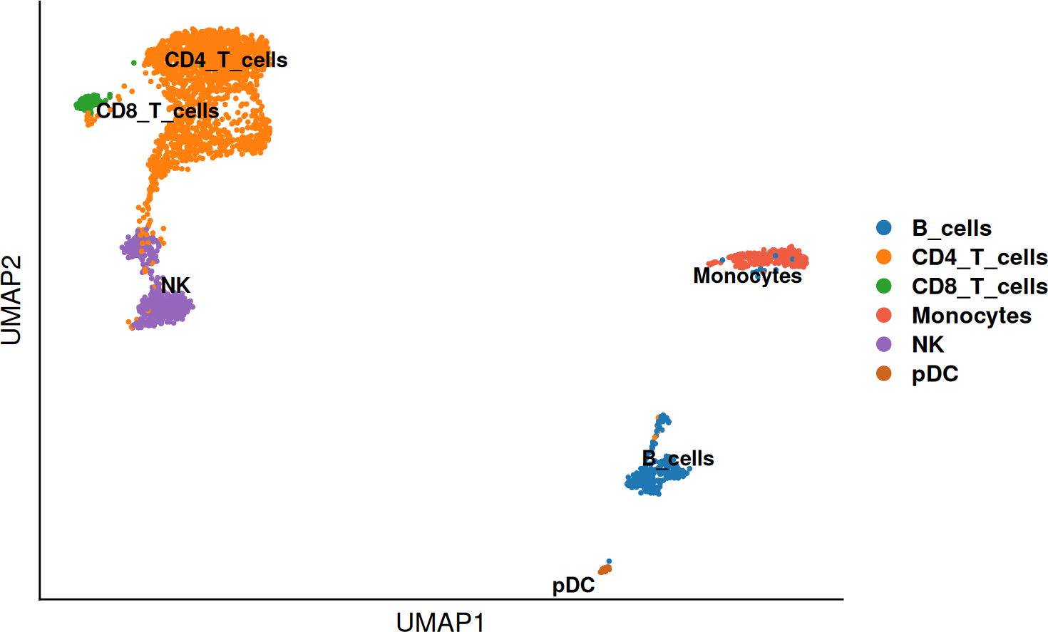
Gene ontology analysis
To explore which biological processes are enriched in a specific cell type across conditions, we can perform gene ontology analysis. We’ll start by identifying differentially expressed genes, focusing here on T cells. For differential gene expression analysis, we introduced a new function, which combines DGE analysis using a single cell approach, e.g. the popular Wilcoxon or MAST test and a pseudobulk testing using DESeq2 or glmGamPoi. We can then observe the results in a combined dataframe.
# this data set contains only one sample per condition
# we introduce replicates for showing the pseudo bulk approach
set.seed(123)
SCE_obj$orig.ident2 <- sample(rep(c("A", "B", "C", "D", "E", "F"),
    length.out = ncol(SCE_obj)
))
CD4T_cells <- DO.Subset(SCE_obj,
    ident = "annotation",
    ident_name = "CD4_T_cells"
)
#> 2026-06-12 10:56:00 - Specified 'ident_name': expecting a categorical variable.

DGE_result <- DO.MultiDGE(CD4T_cells,
    sample_col = "orig.ident2",
    method_sc = "wilcox", #MAST or any test supported by FindMarker function
    method_pb = "DESeq2", # or glmGamPoi
    ident_ctrl = "healthy"
)
#> The following grouping variables have 1 value and will be ignored: annotation
#> Centering and scaling data matrix
#> 2026-06-12 10:56:00 - Annotation names are consistent between original and pseudo-bulk objects.
#> 2026-06-12 10:56:00 - Starting DGE single cell method analysis
#> 2026-06-12 10:56:00 - Comparing disease with healthy in: CD4_T_cells
#> 2026-06-12 10:56:02 - Finished DGE single cell method analysis
#> 2026-06-12 10:56:02 - Starting DGE pseudo bulk method analysis
#> 2026-06-12 10:56:02 - Finished DGE pseudo bulk method analysis
#> 2026-06-12 10:56:02 - DGE pseudo bulk result is empty...

head(DGE_result, 10) %>%
    kable(format = "html", table.attr = "style='width:100%;'") %>%
    kable_styling(bootstrap_options = c(
        "striped",
        "hover",
        "condensed",
        "responsive"
))| gene | pct.1 | pct.2 | celltype | condition | avg_log2FC_PB_DESeq2 | avg_log2FC_SC_wilcox | p_val_adj_PB_DESeq2 | p_val_adj_SC_wilcox | p_val_PB_DESeq2 | p_val_SC_wilcox |
|---|---|---|---|---|---|---|---|---|---|---|
| RGS1 | 0.823 | 0.056 | CD4_T_cells | disease | NA | 5.985999 | NA | 0 | NA | 0 |
| SRGN | 0.977 | 0.489 | CD4_T_cells | disease | NA | 4.036209 | NA | 0 | NA | 0 |
| ZFP36 | 0.935 | 0.418 | CD4_T_cells | disease | NA | 3.690157 | NA | 0 | NA | 0 |
| FOS | 0.962 | 0.587 | CD4_T_cells | disease | NA | 3.234824 | NA | 0 | NA | 0 |
| RGCC | 0.862 | 0.321 | CD4_T_cells | disease | NA | 3.416695 | NA | 0 | NA | 0 |
| ACTB | 0.977 | 0.998 | CD4_T_cells | disease | NA | -1.930151 | NA | 0 | NA | 0 |
| NR4A2 | 0.565 | 0.072 | CD4_T_cells | disease | NA | 3.896930 | NA | 0 | NA | 0 |
| KLF6 | 0.904 | 0.426 | CD4_T_cells | disease | NA | 2.707374 | NA | 0 | NA | 0 |
| AREG | 0.446 | 0.031 | CD4_T_cells | disease | NA | 4.782775 | NA | 0 | NA | 0 |
| ATF3 | 0.323 | 0.002 | CD4_T_cells | disease | NA | 8.336005 | NA | 0 | NA | 0 |
After inspecting the DGE analysis, we continue with
DO.enrichR function, which uses the enrichR API to run gene
set enrichment. It separates the DE genes into up- and down-regulated
sets and runs the analysis for each group independently.
result_GO <- DO.enrichR(
    df_DGE = DGE_result,
    gene_column = "gene",
    pval_column = "p_val_adj_SC_wilcox",
    log2fc_column = "avg_log2FC_SC_wilcox",
    pval_cutoff = 0.05,
    log2fc_cutoff = 0.25,
    path = NULL,
    filename = "",
    species = "Human",
    go_catgs = "GO_Biological_Process_2023"
)
#> Connection changed to https://maayanlab.cloud/Enrichr/
#> Connection is Live!
#> Uploading data to Enrichr... Done.
#>   Querying GO_Biological_Process_2023... Done.
#> Parsing results... Done.
#> Uploading data to Enrichr... Done.
#>   Querying GO_Biological_Process_2023... Done.
#> Parsing results... Done.

head(result_GO, 5) %>%
    kable(format = "html", table.attr = "style='width:100%;'") %>%
    kable_styling(bootstrap_options = c(
        "striped",
        "hover",
        "condensed",
        "responsive"
))| Term | Overlap | P.value | Adjusted.P.value | Old.P.value | Old.Adjusted.P.value | Odds.Ratio | Combined.Score | Genes | Database | State |
|---|---|---|---|---|---|---|---|---|---|---|
| Regulation Of Apoptotic Process (GO:0042981) | 23/705 | 0 | 2.0e-07 | 0 | 0 | 6.105060 | 138.78136 | TOP2A;EGR1;JUN;EGR3;ANXA1;GADD45B;HSPA5;CITED2;IGFBP3;PLAUR;TNF;DUSP6;GADD45G;RHOB;BCL2L11;BCL6;PMAIP1;PIM3;SGK1;PHLDA1;HSPA1B;MCL1;HSPA1A | GO_Biological_Process_2023 | enriched |
| Regulation Of Transcription By RNA Polymerase II (GO:0006357) | 37/2028 | 0 | 2.2e-06 | 0 | 0 | 3.611687 | 70.82183 | CEBPB;CITED2;RORA;PRDM1;TNF;ZFP36;NAMPT;RBBP8;NLRP3;HES4;KDM6B;KLF10;EGR1;JUN;EGR3;TET2;IRF2BP2;FOS;ETV3;SAP30;FOSL2;NR4A2;NFKBIA;NR4A1;KLF6;MAF;RGCC;NR4A3;BCL6;IRF4;ID2;ID1;REL;ID3;FOSB;ATF3;HSPA1A | GO_Biological_Process_2023 | enriched |
| Positive Regulation Of Programmed Cell Death (GO:0043068) | 13/245 | 0 | 3.3e-06 | 0 | 0 | 9.486735 | 178.39945 | TOP2A;JUN;GADD45B;IGFBP3;TNF;DUSP6;GADD45G;RHOB;BCL2L11;BCL6;PMAIP1;PHLDA1;MCL1 | GO_Biological_Process_2023 | enriched |
| Response To Glucocorticoid (GO:0051384) | 6/26 | 0 | 4.8e-06 | 0 | 0 | 48.417073 | 878.20166 | ZFP36;BCL2L11;ANXA1;TNF;ZFP36L2;ZFP36L1 | GO_Biological_Process_2023 | enriched |
| Positive Regulation Of Apoptotic Process (GO:0043065) | 13/270 | 0 | 6.3e-06 | 0 | 0 | 8.552999 | 150.93612 | TOP2A;JUN;GADD45B;IGFBP3;TNF;DUSP6;GADD45G;RHOB;BCL2L11;BCL6;PMAIP1;PHLDA1;MCL1 | GO_Biological_Process_2023 | enriched |
The top significant results can then be visualized in a bar plot.
result_GO_sig <- result_GO[result_GO$Adjusted.P.value < 0.05, ]
result_GO_sig$celltype <- "CD4T_cells"

DO.SplitBarGSEA(
    df_GSEA = result_GO_sig,
    term_col = "Term",
    col_split = "Combined.Score",
    cond_col = "State",
    pos_cond = "enriched",
    showP = FALSE,
    path = paste0(base, "/")
)
GSEA_plot <- list.files(
    path = base,
    pattern = "SplitBar.*\\.svg$",
    full.names = TRUE,
    recursive = TRUE
)
plot(magick::image_read_svg(GSEA_plot))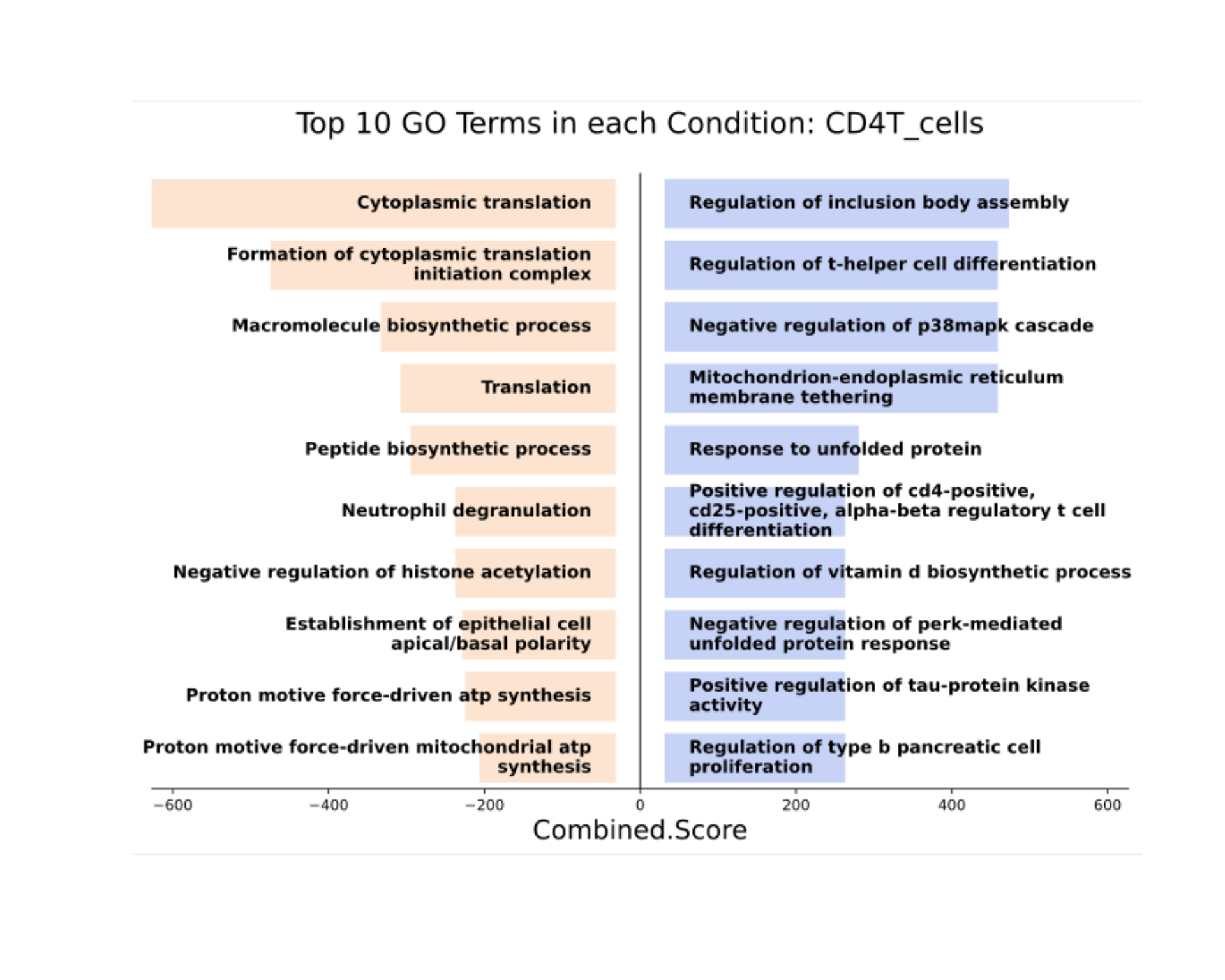
Candidate gene visualisation
After performing DGE and GO analyses, discovering whether specific genes are regulated in a particular disease state and/or cell type is a common step. To address this, we implemented advanced methods in our functions that provide summarised results and incorporate statistical testing to answer these questions efficiently.
The DO.Dotplot function covers the expression over three
variables at the same time along with statistical testing. For example,
we can visualise the expression of a gene across cell types and
conditions:
DO.Dotplot(
    sce_object = SCE_obj,
    group.by.x = "condition",
    group.by.y = "annotation",
    Feature = "NKG7",
    stats_y = TRUE
)
#> Calculating cluster B_cells
#> Calculating cluster CD4_T_cells
#> Calculating cluster Monocytes
#> Calculating cluster NK
#> Calculating cluster pDC
#> Calculating cluster T_cells_5
#> Calculating cluster B_cells
#> Calculating cluster CD4_T_cells
#> Calculating cluster CD8_T_cells
#> Calculating cluster Monocytes
#> Calculating cluster NK
#> Calculating cluster pDC
#> Scale for size is already present.
#> Adding another scale for size, which will replace the existing scale.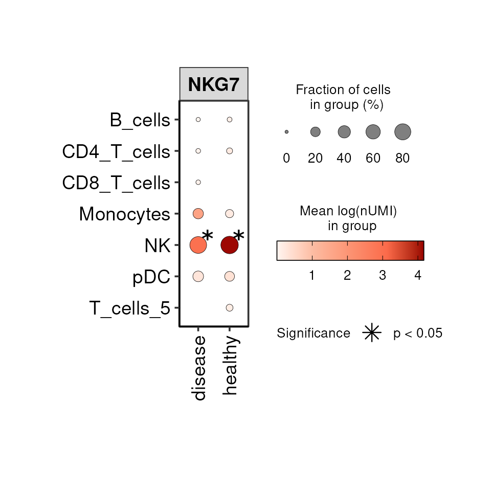
The DO.Heatmap function shows the expression of multiple
genes in a publish ready way, including statistical testing:
path_file <- tempfile("dotools_plots_")
dir.create(path_file, recursive = TRUE, showWarnings = FALSE)

DO.Heatmap(SCE_obj,
    group_by = "leiden0.3",
    features = rownames(SCE_obj)[1:10],
    xticks_rotation = 45,
    path = path_file,
    stats_x_size = 20,
    showP = FALSE,
    figsize = c(8,9)
)
#> Calculating cluster 1
#> Calculating cluster 2
#> Calculating cluster 3
#> Calculating cluster 4
#> Calculating cluster 5
#> Calculating cluster 6
#> Calculating cluster 7
#> Calculating cluster 8

Heatmap_plot <- list.files(
    path = path_file,
    pattern = "Heatmap*\\.svg$",
    full.names = TRUE,
    recursive = TRUE
)

plot(magick::image_read_svg(Heatmap_plot))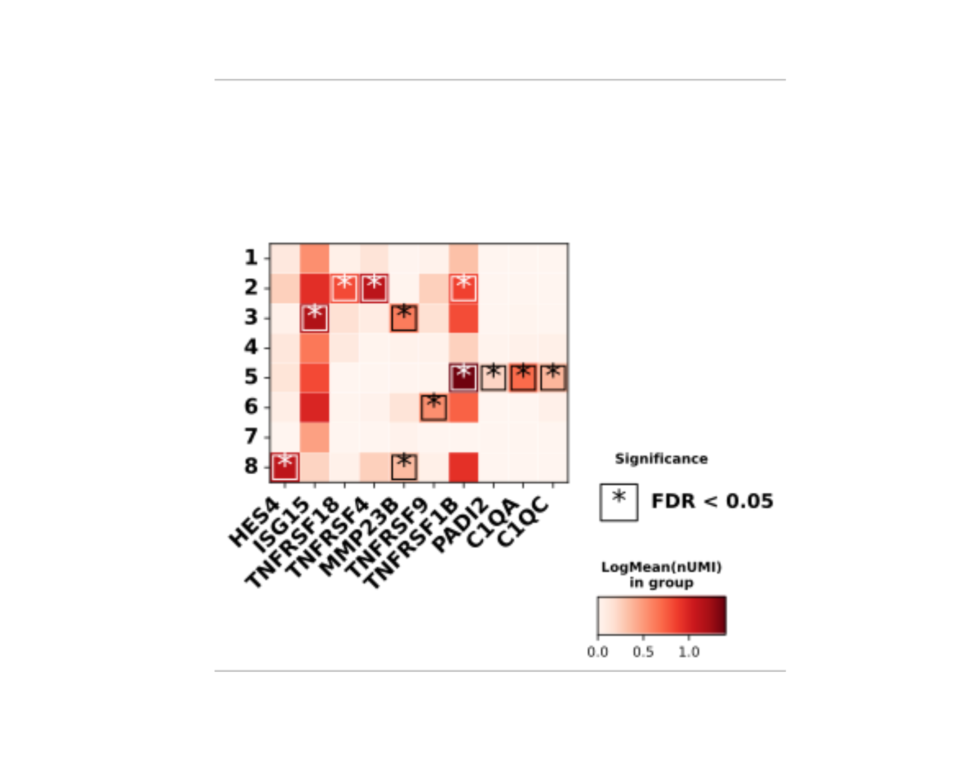
The DO.HeatmapFC function shows the foldchange of
expressions of multiple genes in defined groups in a publication ready
way and still keeping statistical testing for an all-in-one
presentation:
path_file <- tempfile("dotools_plots_")
dir.create(path_file, recursive = TRUE, showWarnings = FALSE)

DO.HeatmapFC(SCE_obj,
    group_by = "leiden0.3",
    features = rownames(SCE_obj)[1:10],
    reference = "healthy",
    condition_key = "condition",
    xticks_rotation = 45,
    path = path_file,
    stats_x_size = 30,
    showP = FALSE,
    ticks_fontproperties = list(size = 14),
    figsize = c(8,7)
)

Heatmap_plot2 <- list.files(
    path = path_file,
    pattern = "Heatmap*\\.svg$",
    full.names = TRUE,
    recursive = TRUE
)

plot(magick::image_read_svg(Heatmap_plot2))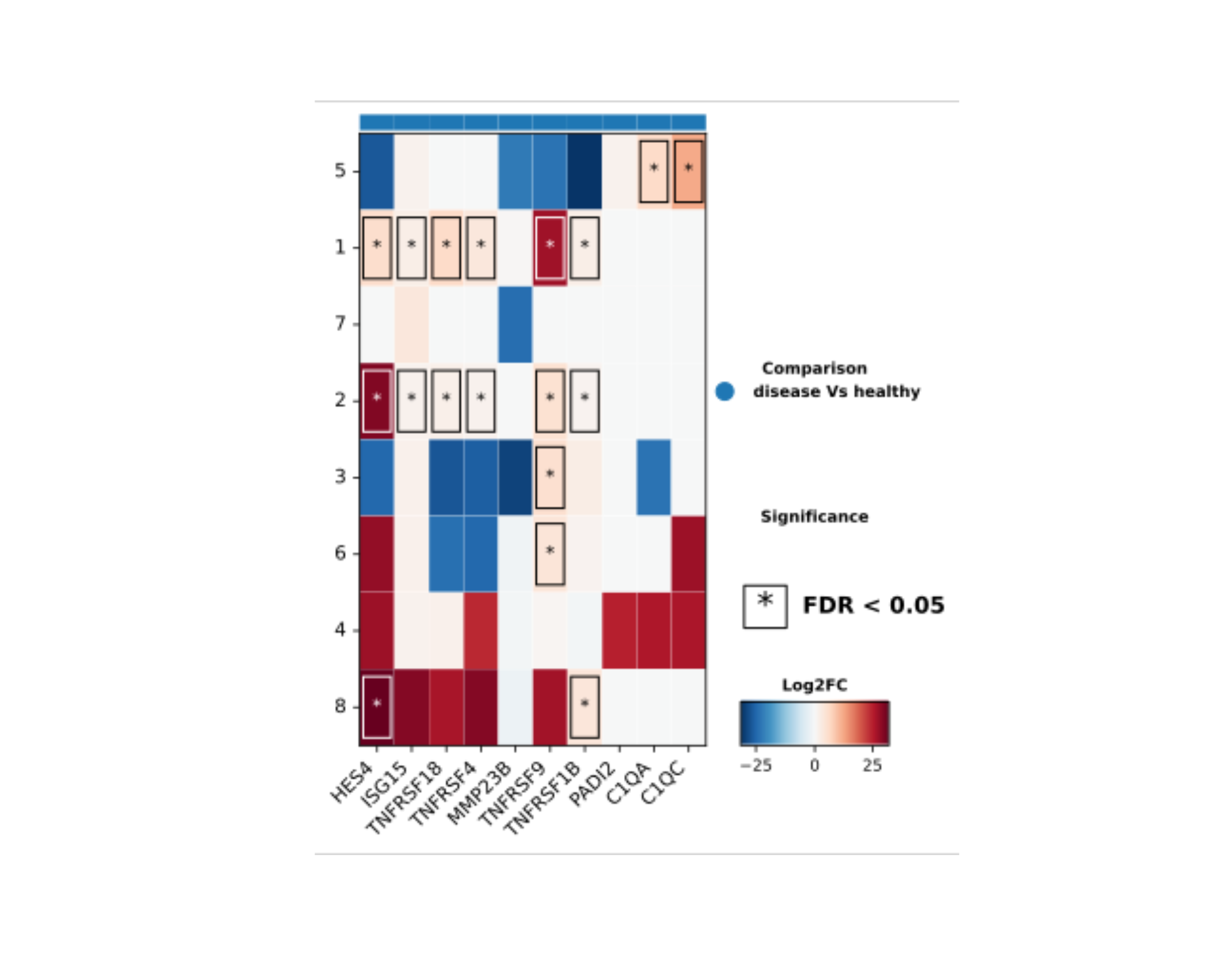
We can visualize the average expression of a gene in a cell type + condition or we can plot continuous metadata information across conditions with violinplots, barplots and boxplots. Additionally, we can test for significance.
SCE_obj_sub <- DO.Subset(SCE_obj,
    ident = "annotation",
    ident_name = c("NK", "CD4_T_cells", "B_cells")
)
#> 2026-06-12 10:56:54 - Specified 'ident_name': expecting a categorical variable.

DO.VlnPlot(SCE_obj_sub,
    Feature = "NKG7",
    group.by = "condition",
    group.by.2 = "annotation",
    ctrl.condition = "healthy"
)
#> Using condition, orig.ident, annotation as id variables
#> 2026-06-12 10:56:54 - ListTest empty, comparing every sample with each other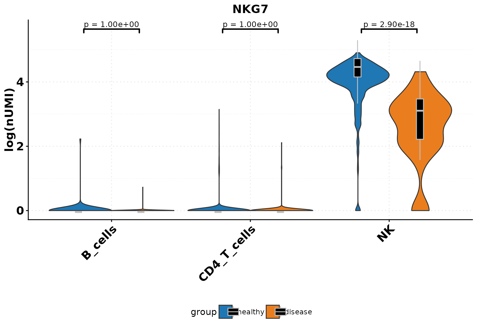
SCE_obj_NK <- DO.Subset(SCE_obj,
    ident = "annotation",
    ident_name = "NK"
)
#> 2026-06-12 10:56:57 - Specified 'ident_name': expecting a categorical variable.

DO.Barplot(SCE_obj_NK,
    group.by = "condition",
    ctrl.condition = "healthy",
    Feature = "NKG7",
    test_use = "wilcox",
    correction_method = "fdr",
    x_label_rotation = 0
)
#> Using condition, orig.ident as id variables
#> 2026-06-12 10:56:58 - ListTest empty, comparing every sample with each other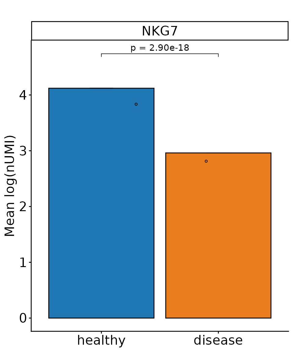
set.seed(123)
SCE_obj$rdm_sample <- sample(rep(c("A", "B", "C"),
    length.out = ncol(SCE_obj)
))

SCE_obj$LogCounts <- log1p(SCE_obj$nCount_RNA)

DO.BoxPlot(SCE_obj,
    group.by = "rdm_sample",
    ctrl.condition = "A",
    Feature = "LogCounts",
    step_mod = 0.01,
    stat_pos_mod = 1.001,
    plot_sample = FALSE
)
#> Using group, cluster as id variables
#> 2026-06-12 10:56:59 - ListTest empty, comparing every sample with each other
#> Scale for fill is already present.
#> Adding another scale for fill, which will replace the existing scale.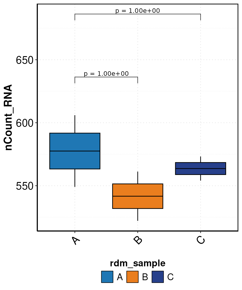
Session information
#> ─ Session info ───────────────────────────────────────────────────────────────────────────────────────────────────────
#>  setting  value
#>  version  R version 4.6.0 (2026-04-24)
#>  os       Ubuntu 24.04.4 LTS
#>  system   x86_64, linux-gnu
#>  ui       X11
#>  language en
#>  collate  C.UTF-8
#>  ctype    C.UTF-8
#>  tz       UTC
#>  date     2026-06-12
#>  pandoc   3.8.3 @ /opt/hostedtoolcache/pandoc/3.8.3/x64/ (via rmarkdown)
#>  quarto   NA
#>
#> ─ Packages ───────────────────────────────────────────────────────────────────────────────────────────────────────────
#>  package              * version   date (UTC) lib source
#>  abind                  1.4-8     2024-09-12 [1] RSPM
#>  assertthat             0.2.1     2019-03-21 [1] RSPM
#>  backports              1.5.1     2026-04-03 [1] RSPM
#>  basilisk               1.24.0    2026-04-28 [1] Bioconduc~
#>  beachmat               2.28.0    2026-04-28 [1] Bioconduc~
#>  beeswarm               0.4.0     2021-06-01 [1] RSPM
#>  Biobase              * 2.72.0    2026-04-28 [1] Bioconduc~
#>  BiocGenerics         * 0.58.1    2026-05-14 [1] Bioconduc~
#>  BiocManager            1.30.27   2025-11-14 [1] RSPM
#>  BiocNeighbors          2.6.0     2026-04-28 [1] Bioconduc~
#>  BiocParallel           1.46.0    2026-04-29 [1] Bioconduc~
#>  BiocSingular           1.28.0    2026-04-28 [1] Bioconduc~
#>  BiocStyle            * 2.40.0    2026-04-28 [1] Bioconduc~
#>  bluster                1.22.0    2026-04-28 [1] Bioconduc~
#>  bookdown               0.46      2025-12-05 [1] RSPM
#>  broom                  1.0.13    2026-05-14 [1] RSPM
#>  bslib                  0.11.0    2026-05-16 [1] RSPM
#>  cachem                 1.1.0     2024-05-16 [1] RSPM
#>  car                    3.1-5     2026-02-03 [1] RSPM
#>  carData                3.0-6     2026-01-30 [1] RSPM
#>  cli                    3.6.6     2026-04-09 [1] RSPM
#>  cluster                2.1.8.2   2026-02-05 [3] CRAN (R 4.6.0)
#>  codetools              0.2-20    2024-03-31 [3] CRAN (R 4.6.0)
#>  colorspace             2.1-2     2025-09-22 [1] RSPM
#>  cowplot                1.2.0     2025-07-07 [1] RSPM
#>  crayon                 1.5.3     2024-06-20 [1] RSPM
#>  curl                   7.1.0     2026-04-22 [1] RSPM
#>  data.table             1.18.4    2026-05-06 [1] RSPM
#>  DelayedArray           0.38.2    2026-05-26 [1] Bioconduc~
#>  DelayedMatrixStats     1.34.0    2026-04-28 [1] Bioconduc~
#>  deldir                 2.0-4     2024-02-28 [1] RSPM
#>  desc                   1.4.3     2023-12-10 [1] RSPM
#>  DESeq2                 1.52.0    2026-04-28 [1] Bioconduc~
#>  digest                 0.6.39    2025-11-19 [1] RSPM
#>  dir.expiry             1.20.0    2026-04-28 [1] Bioconduc~
#>  dotCall64              1.2       2024-10-04 [1] RSPM
#>  DOtools              * 1.3.2     2026-06-12 [1] local
#>  dplyr                * 1.2.1     2026-04-03 [1] RSPM
#>  dqrng                  0.4.1     2024-05-28 [1] RSPM
#>  DropletUtils           1.32.0    2026-04-28 [1] Bioconduc~
#>  edgeR                  4.10.1    2026-05-24 [1] Bioconduc~
#>  enrichR              * 3.4       2025-02-02 [1] RSPM
#>  evaluate               1.0.5     2025-08-27 [1] RSPM
#>  farver                 2.1.2     2024-05-13 [1] RSPM
#>  fastDummies            1.7.6     2026-04-22 [1] RSPM
#>  fastmap                1.2.0     2024-05-15 [1] RSPM
#>  filelock               1.0.3     2023-12-11 [1] RSPM
#>  fitdistrplus           1.2-6     2026-01-24 [1] RSPM
#>  FNN                    1.1.4.1   2024-09-22 [1] RSPM
#>  fontBitstreamVera      0.1.1     2017-02-01 [1] RSPM
#>  fontLiberation         0.1.0     2016-10-15 [1] RSPM
#>  fontquiver             0.2.1     2017-02-01 [1] RSPM
#>  forcats                1.0.1     2025-09-25 [1] RSPM
#>  Formula                1.2-5     2023-02-24 [1] RSPM
#>  fs                     2.1.0     2026-04-18 [1] RSPM
#>  future               * 1.70.0    2026-03-14 [1] RSPM
#>  future.apply           1.20.2    2026-02-20 [1] RSPM
#>  gdtools                0.5.1     2026-05-25 [1] RSPM
#>  generics             * 0.1.4     2025-05-09 [1] RSPM
#>  GenomicRanges        * 1.64.0    2026-04-28 [1] Bioconduc~
#>  ggalluvial             0.12.6    2026-02-22 [1] RSPM
#>  ggbeeswarm             0.7.3     2025-11-29 [1] RSPM
#>  ggcorrplot             0.1.4.1   2023-09-05 [1] RSPM
#>  ggiraph                0.9.6     2026-02-21 [1] RSPM
#>  ggiraphExtra           0.3.0     2020-10-06 [1] RSPM
#>  ggplot2              * 4.0.3     2026-04-22 [1] RSPM
#>  ggpubr                 0.6.3     2026-02-24 [1] RSPM
#>  ggrastr                1.0.2     2023-06-01 [1] RSPM
#>  ggrepel                0.9.8     2026-03-17 [1] RSPM
#>  ggridges               0.5.7     2025-08-27 [1] RSPM
#>  ggsignif               0.6.4     2022-10-13 [1] RSPM
#>  ggtext                 0.1.2     2022-09-16 [1] RSPM
#>  globals                0.19.1    2026-03-13 [1] RSPM
#>  glue                   1.8.1     2026-04-17 [1] RSPM
#>  goftest                1.2-3     2021-10-07 [1] RSPM
#>  gridExtra              2.3       2017-09-09 [1] RSPM
#>  gridtext               0.1.6     2026-02-19 [1] RSPM
#>  gtable                 0.3.6     2024-10-25 [1] RSPM
#>  h5mread                1.4.0     2026-04-28 [1] Bioconduc~
#>  HDF5Array              1.40.0    2026-04-28 [1] Bioconduc~
#>  hms                    1.1.4     2025-10-17 [1] RSPM
#>  htmltools              0.5.9     2025-12-04 [1] RSPM
#>  htmlwidgets            1.6.4     2023-12-06 [1] RSPM
#>  httpuv                 1.6.17    2026-03-18 [1] RSPM
#>  httr                   1.4.8     2026-02-13 [1] RSPM
#>  ica                    1.0-3     2022-07-08 [1] RSPM
#>  igraph                 2.3.2     2026-05-29 [1] RSPM
#>  insight                1.5.1     2026-05-21 [1] RSPM
#>  IRanges              * 2.46.0    2026-04-28 [1] Bioconduc~
#>  irlba                  2.3.7     2026-01-30 [1] RSPM
#>  isoband                0.3.0     2025-12-07 [1] RSPM
#>  jquerylib              0.1.4     2021-04-26 [1] RSPM
#>  jsonlite               2.0.0     2025-03-27 [1] RSPM
#>  kableExtra           * 1.4.0     2024-01-24 [1] RSPM
#>  KernSmooth             2.23-26   2025-01-01 [3] CRAN (R 4.6.0)
#>  knitr                  1.51      2025-12-20 [1] RSPM
#>  ks                     1.15.2    2026-05-09 [1] RSPM
#>  labeling               0.4.3     2023-08-29 [1] RSPM
#>  later                  1.4.8     2026-03-05 [1] RSPM
#>  lattice                0.22-9    2026-02-09 [3] CRAN (R 4.6.0)
#>  lazyeval               0.2.3     2026-04-04 [1] RSPM
#>  leidenbase             0.1.37    2026-05-19 [1] RSPM
#>  lifecycle              1.0.5     2026-01-08 [1] RSPM
#>  limma                  3.68.4    2026-05-31 [1] Bioconduc~
#>  listenv                0.10.1    2026-03-10 [1] RSPM
#>  lmtest                 0.9-40    2022-03-21 [1] RSPM
#>  locfit                 1.5-9.12  2025-03-05 [1] RSPM
#>  magick                 2.9.1     2026-02-28 [1] RSPM
#>  magrittr               2.0.5     2026-04-04 [1] RSPM
#>  MASS                   7.3-65    2025-02-28 [3] CRAN (R 4.6.0)
#>  Matrix                 1.7-5     2026-03-21 [3] CRAN (R 4.6.0)
#>  MatrixGenerics       * 1.24.0    2026-04-28 [1] Bioconduc~
#>  matrixStats          * 1.5.0     2025-01-07 [1] RSPM
#>  mclust                 6.1.2     2025-10-31 [1] RSPM
#>  metapod                1.20.0    2026-04-28 [1] Bioconduc~
#>  mgcv                   1.9-4     2025-11-07 [3] CRAN (R 4.6.0)
#>  mime                   0.13      2025-03-17 [1] RSPM
#>  miniUI                 0.1.2     2025-04-17 [1] RSPM
#>  mvtnorm                1.4-1     2026-06-06 [1] RSPM
#>  mycor                  0.1.1     2018-04-10 [1] RSPM
#>  nlme                   3.1-169   2026-03-27 [3] CRAN (R 4.6.0)
#>  openxlsx               4.2.8.1   2025-10-31 [1] RSPM
#>  otel                   0.2.0     2025-08-29 [1] RSPM
#>  parallelly             1.47.0    2026-04-17 [1] RSPM
#>  patchwork              1.3.2     2025-08-25 [1] RSPM
#>  pbapply                1.7-4     2025-07-20 [1] RSPM
#>  pillar                 1.11.1    2025-09-17 [1] RSPM
#>  pkgconfig              2.0.3     2019-09-22 [1] RSPM
#>  pkgdown                2.2.0     2025-11-06 [1] RSPM
#>  plotly                 4.12.0    2026-01-24 [1] RSPM
#>  plyr                 * 1.8.9     2023-10-02 [1] RSPM
#>  png                    0.1-9     2026-03-15 [1] RSPM
#>  polyclip               1.10-7    2024-07-23 [1] RSPM
#>  ppcor                  1.1       2015-12-03 [1] RSPM
#>  pracma                 2.4.6     2025-10-22 [1] RSPM
#>  prettyunits            1.2.0     2023-09-24 [1] RSPM
#>  progress               1.2.3     2023-12-06 [1] RSPM
#>  progressr              0.19.0    2026-03-31 [1] RSPM
#>  promises               1.5.0     2025-11-01 [1] RSPM
#>  purrr                  1.2.2     2026-04-10 [1] RSPM
#>  R.methodsS3            1.8.2     2022-06-13 [1] RSPM
#>  R.oo                   1.27.1    2025-05-02 [1] RSPM
#>  R.utils                2.13.0    2025-02-24 [1] RSPM
#>  R6                     2.6.1     2025-02-15 [1] RSPM
#>  ragg                   1.5.2     2026-03-23 [1] RSPM
#>  RANN                   2.6.2     2024-08-25 [1] RSPM
#>  RColorBrewer           1.1-3     2022-04-03 [1] RSPM
#>  Rcpp                   1.1.1-1.1 2026-04-24 [1] RSPM
#>  RcppAnnoy              0.0.23    2026-01-12 [1] RSPM
#>  RcppHNSW               0.7.0     2026-05-26 [1] RSPM
#>  reshape2               1.4.5     2025-11-12 [1] RSPM
#>  reticulate             1.46.0    2026-04-09 [1] RSPM
#>  rhdf5                  2.56.0    2026-04-28 [1] Bioconduc~
#>  rhdf5filters           1.24.0    2026-04-28 [1] Bioconduc~
#>  Rhdf5lib               2.0.0     2026-04-28 [1] Bioconduc~
#>  rjson                  0.2.23    2024-09-16 [1] RSPM
#>  rlang                  1.2.0     2026-04-06 [1] RSPM
#>  rmarkdown              2.31      2026-03-26 [1] RSPM
#>  ROCR                   1.0-12    2026-01-23 [1] RSPM
#>  RSpectra               0.16-2    2024-07-18 [1] RSPM
#>  rstatix                0.7.3     2025-10-18 [1] RSPM
#>  rstudioapi             0.19.0    2026-06-11 [1] RSPM
#>  rsvd                   1.0.5     2021-04-16 [1] RSPM
#>  rsvg                   2.7.0     2025-09-08 [1] RSPM
#>  Rtsne                  0.17      2023-12-07 [1] RSPM
#>  S4Arrays               1.12.0    2026-04-28 [1] Bioconduc~
#>  S4Vectors            * 0.50.1    2026-05-13 [1] Bioconduc~
#>  S7                     0.2.2     2026-04-22 [1] RSPM
#>  sass                   0.4.10    2025-04-11 [1] RSPM
#>  ScaledMatrix           1.20.0    2026-04-28 [1] Bioconduc~
#>  scales                 1.4.0     2025-04-24 [1] RSPM
#>  scater               * 1.40.1    2026-05-20 [1] Bioconduc~
#>  scattermore            1.2       2023-06-12 [1] RSPM
#>  SCpubr                 3.0.1     2026-01-09 [1] RSPM
#>  scran                * 1.40.0    2026-04-28 [1] Bioconduc~
#>  sctransform            0.4.3     2026-01-10 [1] RSPM
#>  scuttle              * 1.22.0    2026-04-28 [1] Bioconduc~
#>  Seqinfo              * 1.2.0     2026-04-28 [1] Bioconduc~
#>  sessioninfo            1.2.4     2026-06-04 [1] RSPM
#>  Seurat               * 5.5.0     2026-04-22 [1] RSPM
#>  SeuratObject         * 5.4.0     2026-04-11 [1] RSPM
#>  shiny                  1.13.0    2026-02-20 [1] RSPM
#>  SingleCellExperiment * 1.34.0    2026-04-28 [1] Bioconduc~
#>  sjlabelled             1.2.0     2022-04-10 [1] RSPM
#>  sjmisc                 2.8.11    2025-07-30 [1] RSPM
#>  sp                   * 2.2-1     2026-02-13 [1] RSPM
#>  spam                   2.11-4    2026-05-29 [1] RSPM
#>  SparseArray            1.12.2    2026-05-01 [1] Bioconduc~
#>  sparseMatrixStats      1.24.0    2026-04-28 [1] Bioconduc~
#>  spatstat.data          3.1-9     2025-10-18 [1] RSPM
#>  spatstat.explore       3.8-1     2026-05-24 [1] RSPM
#>  spatstat.geom          3.8-1     2026-05-23 [1] RSPM
#>  spatstat.random        3.5-0     2026-05-24 [1] RSPM
#>  spatstat.sparse        3.2-0     2026-05-21 [1] RSPM
#>  spatstat.univar        3.2-0     2026-05-18 [1] RSPM
#>  spatstat.utils         3.2-3     2026-05-10 [1] RSPM
#>  statmod                1.5.2     2026-05-17 [1] RSPM
#>  stringi                1.8.7     2025-03-27 [1] RSPM
#>  stringr                1.6.0     2025-11-04 [1] RSPM
#>  SummarizedExperiment * 1.42.0    2026-04-28 [1] Bioconduc~
#>  survival               3.8-6     2026-01-16 [3] CRAN (R 4.6.0)
#>  svglite                2.2.2     2025-10-21 [1] RSPM
#>  systemfonts            1.3.2     2026-03-05 [1] RSPM
#>  tensor                 1.5.1     2025-06-17 [1] RSPM
#>  textshaping            1.0.5     2026-03-06 [1] RSPM
#>  tibble               * 3.3.1     2026-01-11 [1] RSPM
#>  tidyr                  1.3.2     2025-12-19 [1] RSPM
#>  tidyselect             1.2.1     2024-03-11 [1] RSPM
#>  tidyverse              2.0.0     2023-02-22 [1] RSPM
#>  uwot                   0.2.4     2025-11-10 [1] RSPM
#>  vctrs                  0.7.3     2026-04-11 [1] RSPM
#>  vipor                  0.4.7     2023-12-18 [1] RSPM
#>  viridis                0.6.5     2024-01-29 [1] RSPM
#>  viridisLite            0.4.3     2026-02-04 [1] RSPM
#>  withr                  3.0.2     2024-10-28 [1] RSPM
#>  WriteXLS               6.8.0     2025-05-22 [1] RSPM
#>  xfun                   0.58      2026-06-01 [1] RSPM
#>  xml2                   1.5.2     2026-01-17 [1] RSPM
#>  xtable                 1.8-8     2026-02-22 [1] RSPM
#>  XVector                0.52.0    2026-04-28 [1] Bioconduc~
#>  yaml                   2.3.12    2025-12-10 [1] RSPM
#>  zellkonverter          1.22.0    2026-04-29 [1] Bioconduc~
#>  zip                    3.0.0     2026-06-10 [1] RSPM
#>  zoo                    1.8-15    2025-12-15 [1] RSPM
#>
#>  [1] /home/runner/work/_temp/Library
#>  [2] /opt/R/4.6.0/lib/R/site-library
#>  [3] /opt/R/4.6.0/lib/R/library
#>  * ── Packages attached to the search path.
#>
#> ─ Python configuration ───────────────────────────────────────────────────────────────────────────────────────────────
#>  python:         /home/runner/.cache/R/basilisk/1.24.0/zellkonverter/1.22.0/zellkonverterAnnDataEnv-0.12.3/bin/python
#>  libpython:      /home/runner/.pyenv/versions/3.14.0/lib/libpython3.14.so
#>  pythonhome:     /home/runner/.cache/R/basilisk/1.24.0/zellkonverter/1.22.0/zellkonverterAnnDataEnv-0.12.3:/home/runner/.cache/R/basilisk/1.24.0/zellkonverter/1.22.0/zellkonverterAnnDataEnv-0.12.3
#>  version:        3.14.0 (main, Jun 12 2026, 10:47:15) [GCC 13.3.0]
#>  numpy:          /home/runner/.cache/R/basilisk/1.24.0/zellkonverter/1.22.0/zellkonverterAnnDataEnv-0.12.3/lib/python3.14/site-packages/numpy
#>  numpy_version:  2.3.4
#>
#>  NOTE: Python version was forced by use_python() function
#>
#> ──────────────────────────────────────────────────────────────────────────────────────────────────────────────────────